1. Foreword
Current Large Language Models (LLMs) suffer from a severe form of anterograde amnesia.
The moment pre-training concludes, the model’s synaptic connections freeze. While In-context Learning grants a fleeting form of working memory, this is merely a transient fitting to the prompt. The model remains incapable of transmuting new information into long-term weights without re-initiating the computationally exorbitant pre-training cycle.

Figure 1: Architectural Schematic. A comparative visualisation of a standard Transformer block versus the proposed HOPE module, highlighting the integration of nested learning mechanisms [1].
Google Research's recent paper, Nested Learning (NL) [1], attempts to break this impasse. However, I argue that the paper's primary contribution is not a State-of-the-Art (SOTA) result, but a radical ontological reconstruction:
“Depth” is an illusion. Neural networks are fundamentally a set of Nested Optimisation Loops, distinguished only by their update frequency.
Without this insight, one sees merely another complex Transformer variant; with it, one perceives a unified mathematical universe.
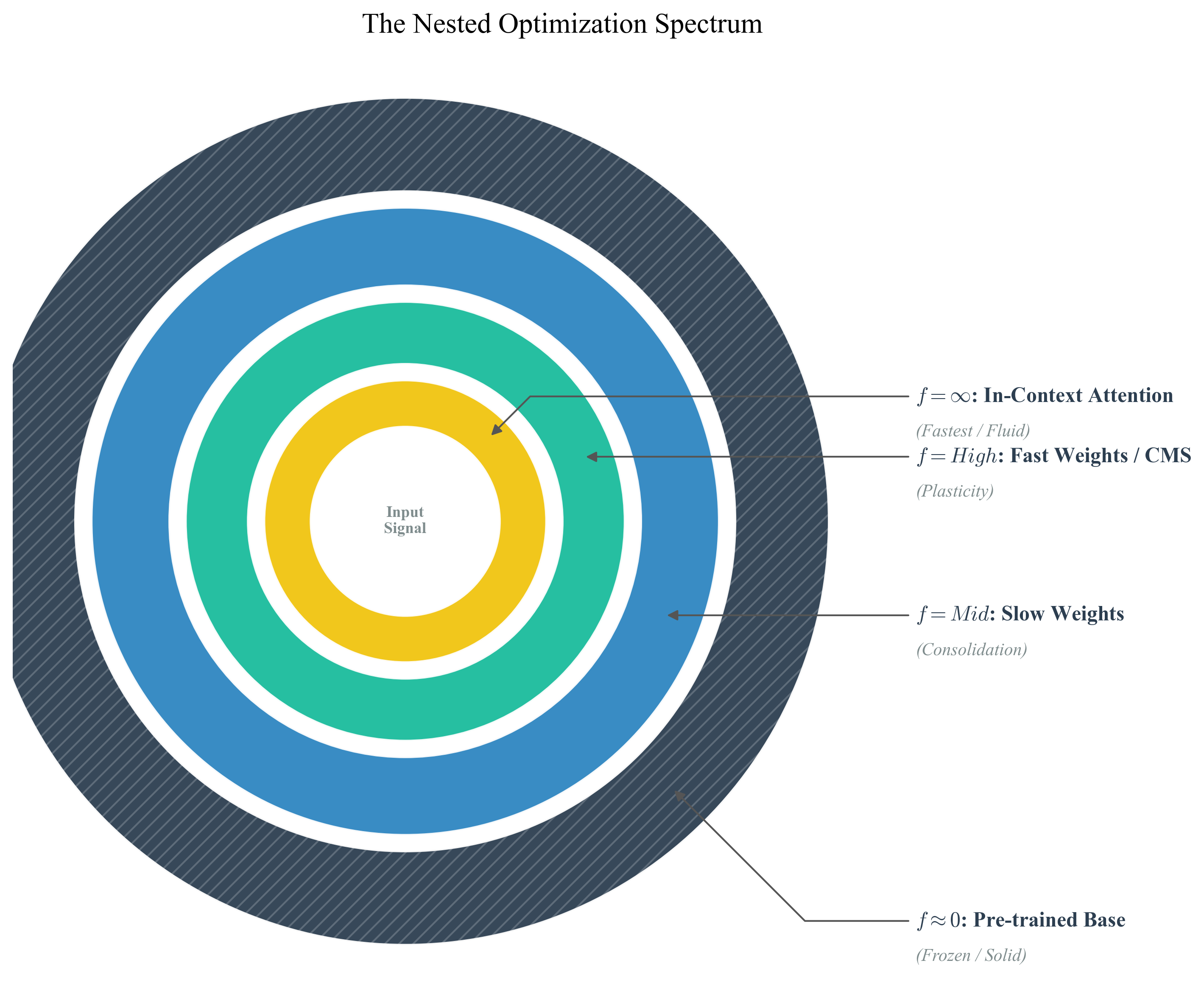
Figure 2: The Nested Optimisation Spectrum. A topological reinterpretation of neural architecture. Instead of vertical depth, layers are viewed as nested loops distinguished by update frequency, ranging from instantaneous In-Context Attention to frozen Pre-trained Weights.
2. Everything is Associative Memory
In the traditional view, the Model and the Optimiser are distinct species.
- Model: $y = f(x; \theta)$ — responsible for inference.
- Optimiser: $\theta_{t+1} = \theta_t - \eta \nabla \mathcal{L}$ — responsible for learning.
Nested Learning presents an elegant mathematical proof: Backpropagation (BP) is itself a self-referential process of associative memory.
Stripping away the notation, the Attention mechanism and Gradient Descent (GD) are mathematically isomorphic. They both perform the same function: information compression.
- Attention ($f=\infty$): Compresses the Context into hidden states via Query-Key matching at the moment of inference.
- SGD ($f \approx 0$): Compresses the Dataset into Weights via Gradient signals over broad epochs.
If one accepts this premise, current architectures leave a massive vacuum between frequencies $0$ and $\infty$. Why, then, do we lack layers operating at $f=10$ or $f=100$?
3. Reconstructing HOPE
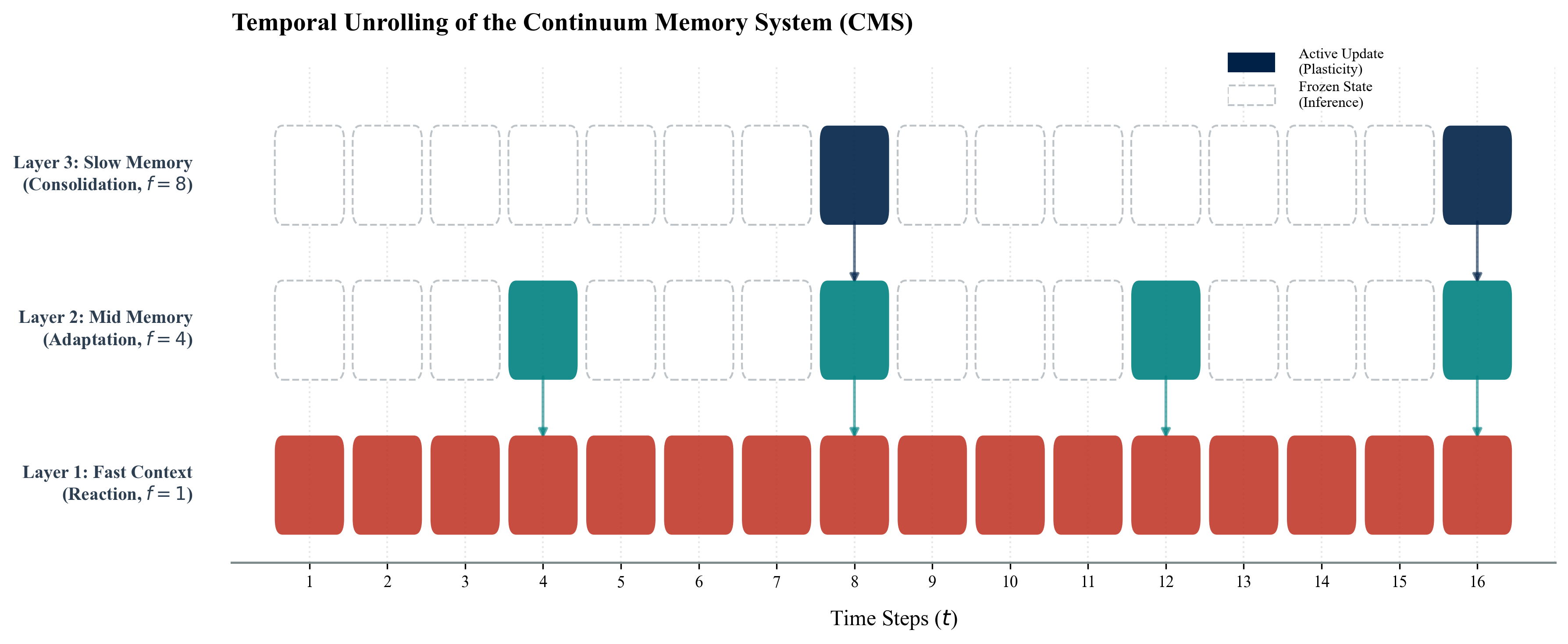
Figure 3: Temporal Unrolling of the Continuum Memory System (CMS). This diagram illustrates the asynchronous update mechanism. Unlike standard synchronous transformers, CMS layers (depicted as horizontal tracks) update conditionally based on their assigned frequency. Solid blocks denote active plasticity, whilst ghosted blocks represent frozen inference states.
Based on this theory, the authors propose the HOPE architecture. Its core component, the Continuum Memory System (CMS) is essentially a differentiable time-divider.
This contradicts the “Synchronous Update” paradigm of the Transformer. CMS allows distinct modules to “breathe” at different rates.
To replicate this in code, one must dissolve the boundary between Training and Inference [3]. Consider the following logic:
The Logic of CMS (Continuum Memory System)
1 | import torch |
The Logic of Self-Modifying Titans [2]
This section often appears esoteric to readers. In Control Theory, however, it is simply adaptive gain.
The model is no longer a passive recipient of a manually tuned Learning Rate; it generates its own parameters based on the “surprise” of the current data. This is effectively Meta-learning at token-level granularity.
1 | class SelfModifyingTitan(nn.Module): |
4. Critical Thoughts
Drawing on OpenReview [4] discussions and experience in High-Performance Computing (HPC), we must examine this technology critically.
Consciousness vs. Smart Cache
Reviewers astutely noted that this mechanism resembles a differentiable smart cache. Fast Layers correspond to L1 Cache (CPU), while Slow Layers correspond to Disk. HOPE simply transforms the Cache into a trainable neural component. While this mitigates Catastrophic Forgetting, it does not fundamentally solve logical reasoning. It simply excels at “rote memorisation”.The Hidden Cost of Sparse Updates
The paper claims CMS is computationally efficient. However, anyone familiar with GPU architectures (e.g., NVIDIA H100) will recognise that logic such asif step % freq == 0is an HPC nightmare.
Warp Divergence: Non-uniform Control Flow causes CUDA Core utilisation to plummet.
Pipeline Bubbles: In distributed training, asynchronous updates render gradient synchronisation (AllReduce) excessively complex.
In deployment, the wall-clock time gains may be significantly lower than the theoretical reduction in FLOPs.
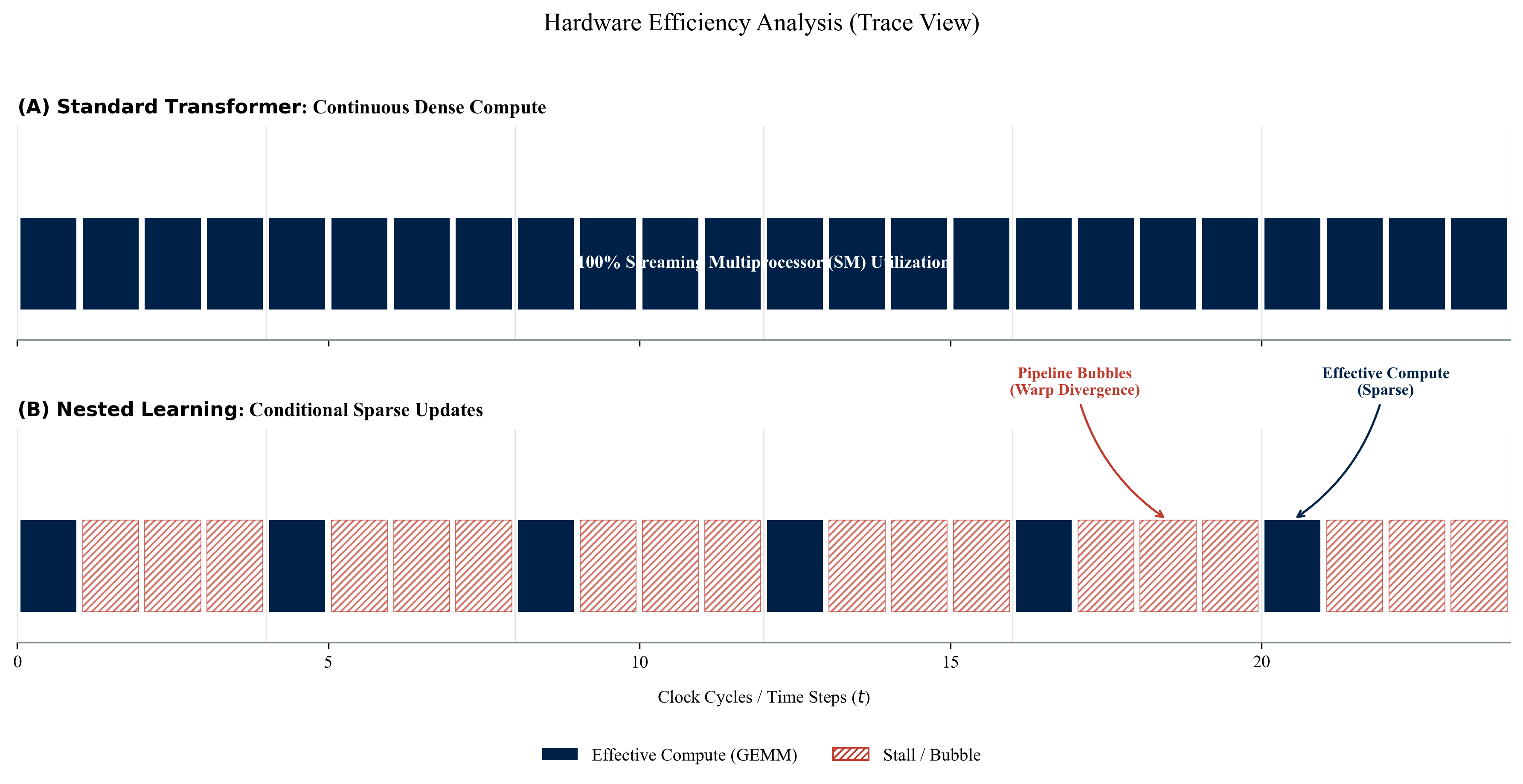
Figure 4: Hardware Efficiency Analysis (Trace View). A comparative profile of GPU pipeline utilisation. Panel (A) shows the dense compute of Standard Transformers, whilst Panel (B) demonstrates how Nested Learning induces 'Pipeline Bubbles' and warp divergence due to conditional sparse updates, highlighting the trade-off between theoretical FLOPs reduction and wall-clock latency.
- Financial Implications: Handling Regime Change
From a Quantitative Finance perspective, Catastrophic Forgetting is simply a regime switch. Traditional LLMs assume a stationary distribution for training data. NL allows the model to adjust local parameters dynamically during inference—essentially online risk adaptation. For high-frequency trading or real-time risk modelling, this capability (“learning while running”) may prove far more disruptive than its applications in NLP.
5. Final Thoughts
Nested Learning acts as a mirror. It reveals that Parameters are not sacred, static entities; they are simply memory variables with an extremely low frequency.
When one writes param.sub_(0.01 * state), one is not merely writing code; one is designing a digital entity with multiple temporal perceptions.
The architectural battles of the future will not be fought over Depth, but over frequency bandwidth.
Copyright Notice
This article, except for the referenced content below, is the original work of Junhao. The author retains the exclusive rights to its final interpretation. If there are any issues regarding copyright infringement, please contact me for removal. Reproduction or distribution of this content without my explicit permission is prohibited.
6. References
[1]. Behrouz, A., Razaviyayn, M., Zhong, P., & Mirrokni, V. (2025). Nested Learning: The Illusion of Deep Learning Architecture. Google Research. The Thirty-ninth Annual Conference on Neural Information Processing Systems (NeurIPS).
[2]. Behrouz, A., Pezeshki, M., et al. (2025). Titans: Learning to Memorize at Test Time. Google Research. arXiv preprint arXiv:2501.00663 (2024).
[3]. Sun, Y., et al. (2020). Test-Time Training with Self-Supervision for Generalization under Distribution Shifts. International Conference on Machine Learning (ICML).
[4]. OpenReview Forum. (2025). Nested Learning: The Illusion of Deep Learning Architecture. Available at: https://openreview.net/forum?id=nbMeRvNb7A